Having recently concluded my seven-part series (see links at the end of this article) on leading asset-management indicators that drive proactive behaviors in maintenance and reliability, I’m now turning my attention to lagging metrics. Think of leading indicators as the cause and lagging indicators as the effect in terms of equipment-asset performance. In this article, the first installment of a short series, the focus is on Mean Time Between/To Failure (MTBF/MTTF).
At first glance, MTBF/MTTF seems obvious. Hold on, though. Not so fast. To be clear, MTBF/MTTF is a relatively complex metric. Let’s explore this further.
MTBF/MTTF BASICS
To start, let’s differentiate MTBF from MTTF. For repairable items, we typically monitor MTBF. For replaceable items, we track MTTF. For example, we would employ MTBF to trend the reliability of a centrifugal pump. However, we would employ MTTF to trend the reliability of the pump’s drive-end (DE) bearing . This brings us to the first complexity of the MTBF/MTTF metric: We need to monitor the reliability of our assets at the system level, the component level, and the part level.
For our centrifugal pump example, we must track the reliability for the system, which, among other things, would typically include the pump, motor, coupling, motor-control center (MCC), inlet piping, and outlet piping. In addition, we must monitor the performance of all those components individually, along with various parts associated with each component’s assembly. So, for the defined-level analysis, calculate MTBF/MTTF by adding the running time/cycles/miles/etc. for failed and unfailed items alike and dividing that sum by the total number of failures observed (Fig. 1).
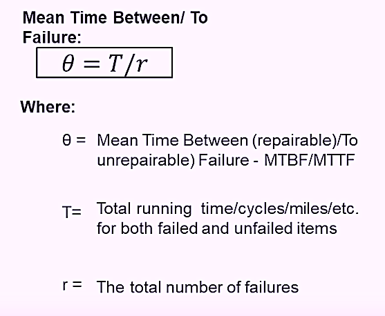
Fig. 1. The formula for calculating MTBF/MTTF.
THE VARIABILITY EFFECT
Average, or the arithmetic mean, is the first moment of the probability distribution. It is a measure of central tendency. Median and mode are also measures of central tendency. When one thinks of the mean, or average value, the familiar bell-shaped curve of the Gaussian distribution comes to mind. When the mean, median, and mode are approximately equal, the distribution is typically bell-shaped. (NOTE: Although there are exceptions to that rule, they’re beyond the scope of this article). A measure of central tendency, such as MTBF/MTTF, without a measure of variability about that mean can be very misleading and lead to poor decisions.
For example, if an asset or component has a MTBF/MTTF of 1,000 operating hours, one might decide to schedule a rebuild or replacement at some time before 1,000 hours (say 800 hours). Without knowledge of the variance, which is the second moment of a probability distribution, a reasonable decision can’t be made about that 1,000-hr. MTBF/MTTF.
From variance, we derive the standard deviation, which is calculated as the square root of the calculated variance. In our example, if the standard deviation about the 1,000-hr. MTBF/MTTF is 70 hours, the decision to rebuild or replace at 800 hours would be a rather good one. That’s because to be 95% confident about taking action before a failure, we would multiply the standard deviation by 1.65 and subtract that from the MTBF/MTTF. Subtracting 115.5 from 1,000 equals 884.5. Therefore, an 800-hr. rebuild or replace decision would be safe.
On the other hand, what happens if the MTBF/MTTF is 1,000 hours and the standard deviation is 700? In this case, we would need to subtract 1,155 from 1,000 to determine a suitable rebuild or replace time. But that results in a negative number. Probabilistically, one would not be able to even start the machine in question. This clearly is not reasonable.
THE RISK PROFILE AS A FUNCTION OF TIME
In addition to considering the variability about the MTBF/MTTF, we must also consider the failure-risk profile as a function of time (Fig. 2). Some machines, including components and their parts, experience a higher risk of failure when they’re new. Such events are sometimes referred to as early-life, infant, or so-called “burn-in” or “run-in” failures. In other instances, we observe a constant risk of failure over time. And in still other cases, the failure rate will gradually increase or geometrically increase as a function of time. Understanding the risk profile as a function of time is essential for making informed and effective asset-management decisions. Those different risk profiles as a function of running time/cycles/miles/etc. create very different probability distributions.
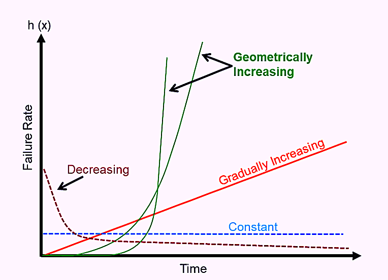
Fig. 2. Different failure risk profiles as a function of time.
LOOK TO WEIBULL ANALYSIS FOR HELP
Reliability engineers employ Weibull analysis to gain an understanding about the risk profile as a function of time for equipment assets, their components, and the parts for those components. An essential output from Weibull analysis is the Beta Shape Parameter (β).
As depicted in Fig. 3, when the β is less than 1.0, the system/component/part/experiences early life failures. The closer the β shape parameter is to zero, the stronger the early-life failure risk. When β is approximately equal to 1.0, the failure rate is constant as a function of time. When β is approximately equal to 2.0, the failure rate is linearly increasing as a function of time, which produces a skewed (Rayleigh distribution. Skew is the third moment of the probability distribution. When the β shape parameter equals about 3.5., the distribution assumes the familiar bell-shape of the normal or Gaussian distribution. As the β shape parameter increases above 3.5, the coefficient of variation decreases, the bell curve tightens up, and the kurtosis, or the peakiness of the curve, i.e., the fourth moment of a probability distribution, increases.
A decision to rebuild or replace an asset, its components, or the parts of those components, based on running time/cycles/miles/etc., only makes sense when the β shape parameter is well above 3.5.
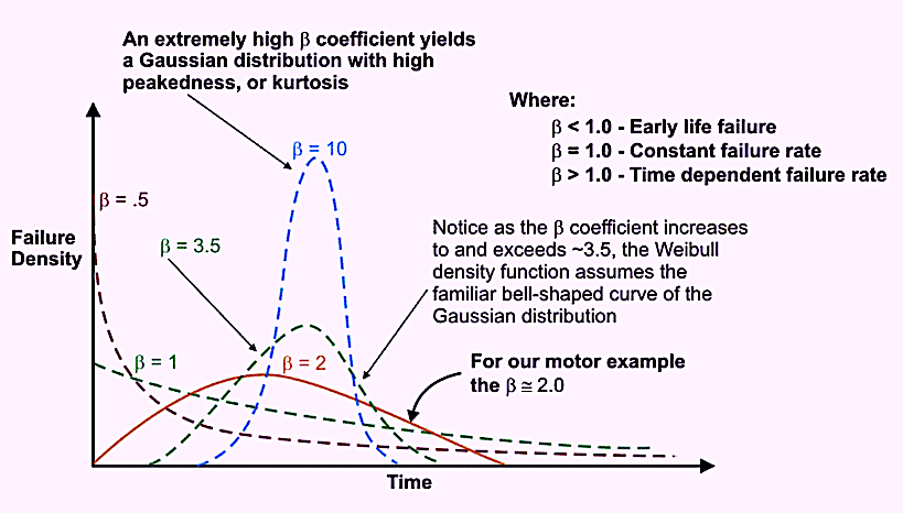
Fig. 3. Various probability distributions for different Beta (β) Shape Parameter values.
CONCLUSIONS
Mean Time Between/To Failure (MTBF/MTTF) is the average, which can be a very misleading (click here to see my article, “As A Metric, ‘Average’ Can Be A Dangerous Number”). Without knowledge about the variability of the average and the risk profile as a function of time, some very poor equipment-asset-management decisions can be made. Also, keep in mind that we must evaluate failure probability at the system, component, and part levels to make smart decisions and ensure effective allocation of asset-care resources (money and time).
Next week, we’ll continue the discussion on MTBF/MTTF by focusing on the effect of different failure modes.TRR
Click Here To Read Articles In This Series On Leading Indicators For Asset Management
“Overall Inspection Effectiveness (OIE)”
“Overall Lubrication Effectiveness (OLE”)
“Overall Vibration Effectiveness (OVE)”
“Overall Electrical Effectiveness (OELE)”
“Overall Planning Effectiveness (OPE)”
“Overall Scheduling Effectiveness (OSE)”
“Overall Materials Effectiveness (OME)”
ABOUT THE AUTHOR
Drew Troyer has over 30 years of experience in the RAM arena. Currently a Principal with T.A. Cook Consultants, he was a Co-founder and former CEO of Noria Corporation. A trusted advisor to a global blue chip client base, this industry veteran has authored or co-authored more than 300 books, chapters, course books, articles, and technical papers and is popular keynote and technical speaker at conferences around the world. Drew is a Certified Reliability Engineer (CRE), Certified Maintenance & Reliability Professional (CMRP), holds B.S. and M.B.A. degrees. Drew, who also earned a Master’s degree in Environmental Sustainability from Harvard University, is very passionate about sustainable manufacturing. Contact him at 512-800-6031, or email dtroyer@theramreview.com.
Tags: reliability, availability, maintenance, RAM, metrics, key performance indicators, KPIs, MTBF, MTFF, Weibull Analysis