Up until now, we’ve focused on just using raw electric-motor data in this Machine Learning series (see article links to below). That includes moving from working through the information to classifying different types of faults with it. The aim, in effect, has been to replicate what we do when we look at this same information and process in our minds. For example, in Part V, we used data classification to detect an unbalance in voltage or current and understand their respective impacts on power factor. This week, with the help of degradation models, we explore the concept behind Remaining Useful Life (RUL), also known as Time to Failure Estimation (TTFE).
Click The Following Links To Read Previous Articles In This Series
Part I (Aug. 8, 2021)
The concepts behind RUL are not far-fetched: They’re basically reliability and industrial-engineering concepts.
♦ The basics behind TTFE for electric machines were introduced in a 2009 IEEE Electrical Insulation Magazine article titles, “Simple Time-to-Failure Estimation Techniques for Reliability and Maintenance of Equipment”[1]. This article described a simple method for predictive-maintenance-time-to-failure estimation for electric machines.
♦ Advanced techniques were subsequently introduced in the IEEE paper, “Evaluating Reliability of Insulation Systems for Electric Machines”[2], that was presented at the 2014 Electrical Insulation Conference. The paper approached TTFE through consideration of multi-factor impacts of electrical, thermal, and mechanical stresses in hybrid vehicles. In each case, aging and risk data were required to provide a risk-based estimate of the remaining machine life.
(For those pursuing a TTFE approach in a real-world predictive-maintenance (PdM) program (be it electrical or mechanical), these two papers are good primers.)
When we know what degradation of a motor looks like, either through historical or modeled data, we can relate it to existing and expected thresholds. There are a variety of approaches to the application of RUL, so the programmer/developer must select the one that fits best. For purposes of this article, we are reviewing two regression-type models: linear and exponential. The descriptions are self-explanatory. If the TTFE degradation is in a straight line, it’s linear. If the degradation is exponential, usually as a natural log, it’s exponential. However, the analyst should take care: There are cases when it could be assumed degradation is either type (such as exponential for temperature), but it actually follows a more linear pattern.
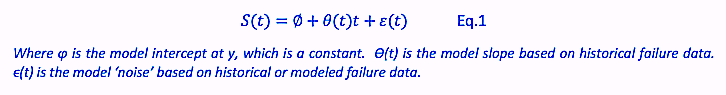
The linear degradation model used within Matlab assumes a continuous-time linear degradation as identified in Equation 1.
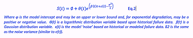
The exponential degradation model also assumes a continuous-time degradation, but as a curve as identified in Equation 2.
While these two degradation models are normally used for continuous-time analysis, they also can be used successfully in variable load, speed, and start/stop applications when good historical or modeled data is applied. De-energizing equipment and allowing it to cool off may reset the time on the electric motor when it is again started. Experience has shown, however, that machine degradation will return to the proper RUL once the machine returns to temperature. If data is available, one reason for selecting these degradation methods is to allow for RUL-time correction when loads, speeds, or other changes are made. Increasing stresses will decrease time to failure, while decreasing them may increase the availability of the machine. There are several other regression systems for RUL that provide flexibility for the developer that you may wish to explore.
Within the Matlab environment, the data we created to classify different types of faults can now be applied to the RUL and RUL training as the training methods are built into the Predictive Maintenance, Machine Learning, and Statistical Processing modules. We will start by creating our linear and exponential framework before we start training them. At this point, we also must consider what timeframe we want to track: days, hours, minutes, or seconds. Tracking “hours” is recommended as a good frequency, because it can be easily adjusted when coding software outputs.
First, we want to verify the Ensemble we created during classification (Part V), as shown in Fig. 1 and Fig. 2 below. This will be our training data.
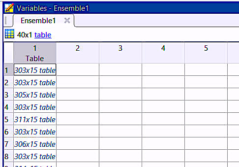
Fig. 1. The ensemble will be a table of training data tables.
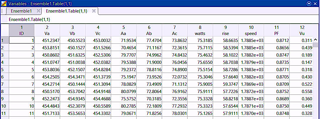
Fig. 2. The data within each of the tables from Fig. 1.
In the next step, we create our regression containers, as shown in Fig. 3. For purposes of our hypothetical ML project, we’re going to handle each variable independently as we will end up taking the shortest measured time to failure as our expected RUL. We need multiple RUL algorithms for this, and they can also be of types with which we work when coding.
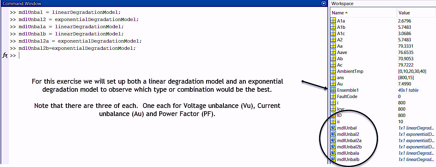
Fig. 3. Voltage unbalance, current unbalance, and power factor in both exponential and linear degradation.
Training our software with both regression models will provide what’s necessary to select the best model for each type of measurement. The remainder can be disgarded before the trained software is ready for use. Each of the developed regression containers shown in Fig. 3 will appear as in Fig. 4.
Nest, we’ll go through each regression container and code in “mdlUnbal = linearDegradationModel(‘LifeTimeUnit’, ‘hours’).” This will update the calculated units. These units should be the same as the data collection, which, in our example, is hourly, and the name of the model should be the name that you’ve already used.
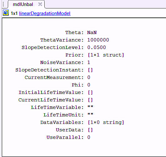
Fig. 4. Pre-training regression container for linear degradation.
The table format used for training the model must be the same as the data that will be fed into the system from the real data. For training each model in Matlab, we use a :fit” command: fit(mdlUnbal,Ensemble1.Table,”ID”,”Au”) where the data from each table in Ensemble1 will be used from “ID”, which we are using to represent hours, and “Au,” which is the variable representing current unbalance.
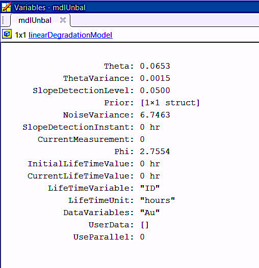
Fig. 5. The linear degradation model following training.
For testing, we work with another set of data using an unbalance and set our current unbalance threshold (thresholdAu) to 20 and our voltage unbalance threshold (thresholdVu) to 6 (which would be 20% and 6% respectively). The trained model will then look at the data and determine the length of time that the degradation would take, based upon the slope of the curve linearly as shown in Fig. 6.
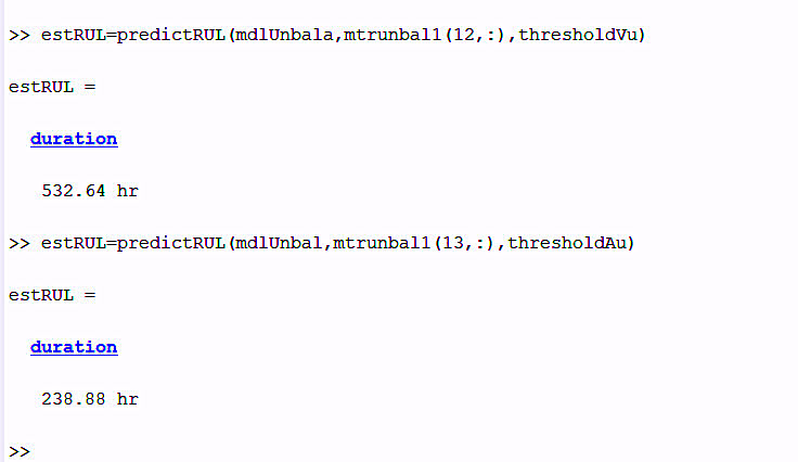
Fig. 6. Testing against “known” failure data to see if the duration matches. In this case,
the selection would be current unbalance, which is the shortest duration.
During testing, Matlab identified that the failure curves didn’t fit exponential degradation, so those would be discarded. Assuming our hypothetical machine would be running at this load and speed constantly, the duration from this test would be ~239 hours or ~10 days at the present rate of degradation based on increasing current unbalance. If this methodology is run hourly, then changes to operation, load, etc., would constantly update the RUL value.
COMING UP
In Part VII, we will assemble the program (function or script) using what we have done so far and include some management advice on avoiding false positives. Note that we are limiting this project to just voltage and current unbalance. A final, real-world program would be a more time- and coding-intensive.
It’s important to keep in mind that the purpose of this series has been to provide readers with an understanding of how Machine Learning works. That said, there are plenty of ML applications beyond the viewing of vibration data.TRR
REFERENCES
1. H. W. Penrose, “Simple Time-to-Failure Estimation Techniques for Reliability and Maintenance of Equipment,” IEEE Electrical Insulation Magazine, Vol. 25, No. 4, pp. 14-18, July-Aug. 2009, doi: 10.1109/MEI.2009.5191412.
2. H. W. Penrose, “Evaluating Reliability of Insulation Systems for Electric Machines,” 2014 IEEE Electrical Insulation Conference (EIC), 2014, pp. 421-424, doi: 10.1109/EIC.2014.6869422.
ABOUT THE AUTHOR
Howard Penrose, Ph.D., CMRP, is Founder and President of Motor Doc LLC, Lombard, IL and, among other things, a Past Chair of the Society for Reliability and Maintenance Professionals, Atlanta (smrp.org). Email him at howard@motordoc.com, or info@motordoc.com, and/or visit motordoc.com.
Tags: reliability, availability, maintenance, RAM, electrical systems, electric motors, ML, artificial intelligence, AI, Electrical Signature Analysis, ESA, Motor Current Signature Analysis, MCSA, predictive maintenance, PdM, preventive maintenance, PM, Matlab, mathworks.com, python.org