
In Part IV of this series (link below), we determined how to pre-process data for our example Machine Learning (ML) project. Here, we discuss development of data representing defective conditions if the real-world type isn’t available. Beware, though: This task can be a rather time-consuming endeavor. It also requires some experience in what happens to different variables when defects occur.
Click The Following Links To Read Previous Articles In This Series
Part I (Aug. 8, 2021)
For this article, we’re using the example of a voltage unbalance and focusing on three areas associated with that it: voltage unbalance in phase A; current unbalance in phase A; and, power factor. There are additional considerations, including, for example, temperature rise due to the unbalance, which would force de-rating of the motor, and possible vibration changes, which we will not cover here.
The first step is to automate the development of our fault data, which can be accomplished through progressive random-number-generation modifications to the original script (learn more in the Sidebar at the end of this article) followed by pre-processing. For the purposes of this article, we’ve created 10 sets of “good” csv files and 10 sets of voltage-unbalance csv files. The code to create the voltage unbalance also updates the “FaultCode” variable and ends the file creation at the point the motor is considered “failed.” This will provide the information to create the fault classification, which we are covering in this article, and provides the data to help develop the Remaining Useful Life (RUL) algorithm, which will be discussed in our next article.
Having selected Matlab software for the development of our ML tool, after pre-processing the training data, we import it as shown in Fig. 1. When we perform this step, we identify the independent variables, such as time, and condition variables, such as FaultCode. In this case, we’re importing all good and bad data with FaultCodes so the software can help identify features of each type of defect.
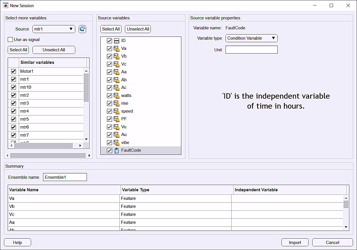
Fig. 1. Matlab PdM tool Diagnostic Feature Designer (DFD) import screen.
The Matlab Diagnostic Feature Designer (DFD) shown in Fig. 2 is the part of a toolbox that helps the data scientist select the order of features through different statistical techniques. For supervised systems, such as in this case, ranking of the features is performed with either the One-Way ANOVA (Analysis of Variance for Linear Regression Model to compare populations of data that have a normal distribution), or with the Kruskal-Wallis test (a version of the one-way ANOVA that compares the median values of more than two groups to determine if they are from the same population). Good values are scored over 100, with the highest values representing the best features for classification.
When we look at such data, it should be apparent that we generated the voltage unbalance strictly on one phase and the associated current unbalance. We also should also be able to see that the highest values are in the straight One-Way ANOVA process in the top five sets of data. First, we should realize that if we include the features for voltage and current phase A it will only detect and classify those conditions where we have an unbalance in Phase A. The correction would be addition of training data that have unbalances and variations in each of the other phases, or removal of the voltage and current data and use of just the change in unbalance (Vu and Au) and power factor.
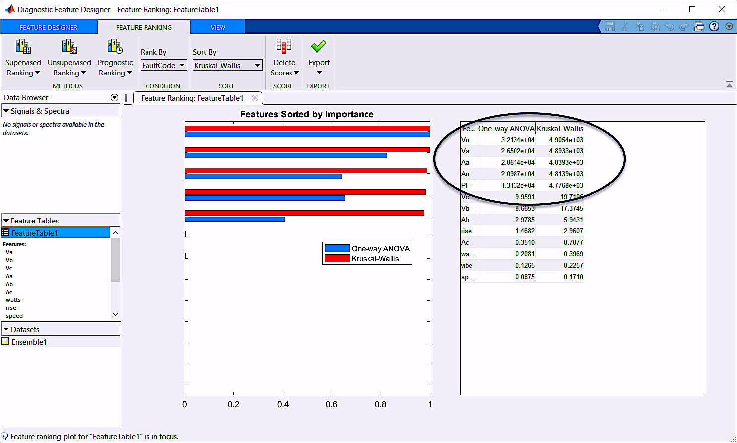
Fig. 2. Matlab Diagnostic Feature Designer Tool (DFD).
In the next step (Fig. 3), the DFD also allows us to export all training data as a single ensemble (listing of tables) that can be used in other parts of our work including RUL. While developing these ensembles can be performed manually later on, this software capability will save time, especially since we will want to use the same data in both Classification and RUL.
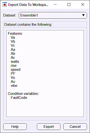
Fig. 3. Ensemble export in the Matlab DFD.
Following the identification of features within the data, we would then export it to the Matlab Classification Learner Application (CLA) that lets us select and train the classification algorithm (Fig. 4). In this step, as noted in Fig. 4, we only need three data features and fault code out of all the data we used in the DFD application. (NOTE: For those using software such as Python, R, or other open-source or commercial systems, much of this step may be done through coding. In these cases, development can be automated or different packages applied).
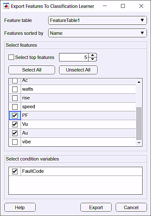
Fig. 4. Export to the Matlab Classification Learner Application (CLA).
As shown in Fig. 5, a form of pre-processing is again performed during the CLA data setup. Several methods can be used to validate and process the input data. In this case, the FaultCode is used to identify the conditions associated with the data that result in classification based upon the model; and the predictors are used in the development of the model based upon the DFD step.
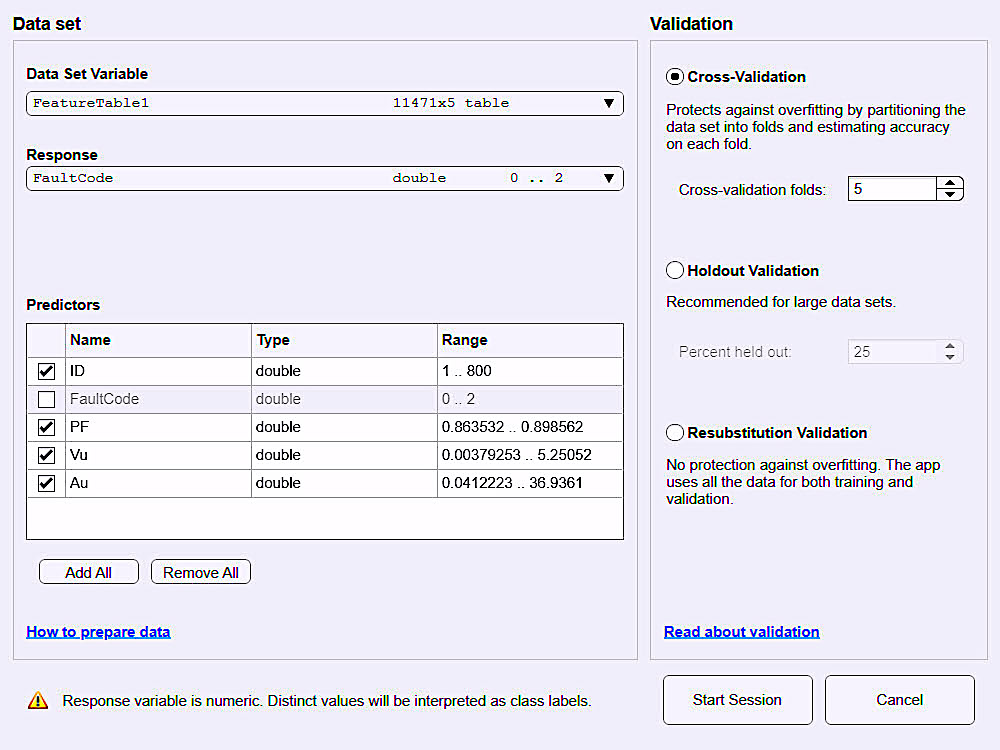
Fig. 5. Matlab CLA data setup and pre-processing.
As depicted in Fig. 6, once the data is imported to the CLA, you can select the types of algorithms you wish to train and test. In this case, we’ve selected all methods, have left all additional capabilities in default, and then selected “Train.” This permits the CLA to use variations of the provided data to train the output algorithms and verify their accuracy against the known FaultCodes. The algorithms will range from “Trees” (basically fault trees), to nearest known neighbors and neural networks, which would be used in our final classification model.
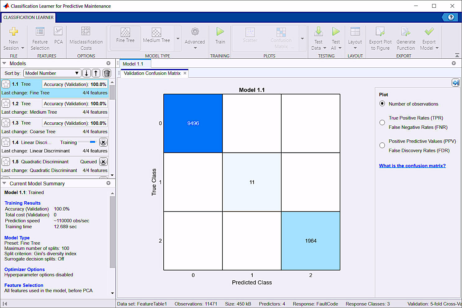
Fig. 6. Matlab CLA training and testing of the algorithms.
The CLA provides a variety of tools and processes to evaluate data visually (Fig. 7) and determine its accuracy, as well as allow weighting of different methods for greater accuracy. In the end, every step performed can be exported to Matlab script or functions. This documents the process for obtaining the final data and ensures that it can be repeated.
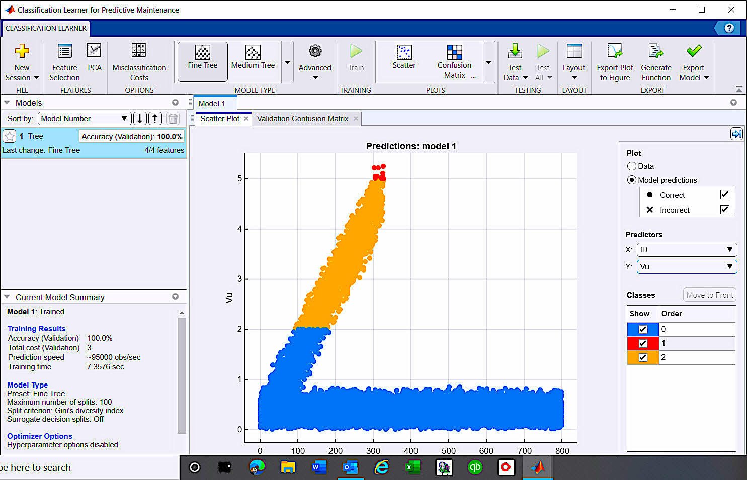
Fig. 7. CLA scatter plot shows 2% unbalance generating alarm, and 5% unbalance observed as failure.
Once the classification algorithm is trained and tested, we can then export it into a trained model that can be used to perform analysis on new data, as shown in Fig. 8. The trained model can be exported with all training data or with just the algorithm. At this point, we generally test the trained algorithm on known data, but not on the original tested data.
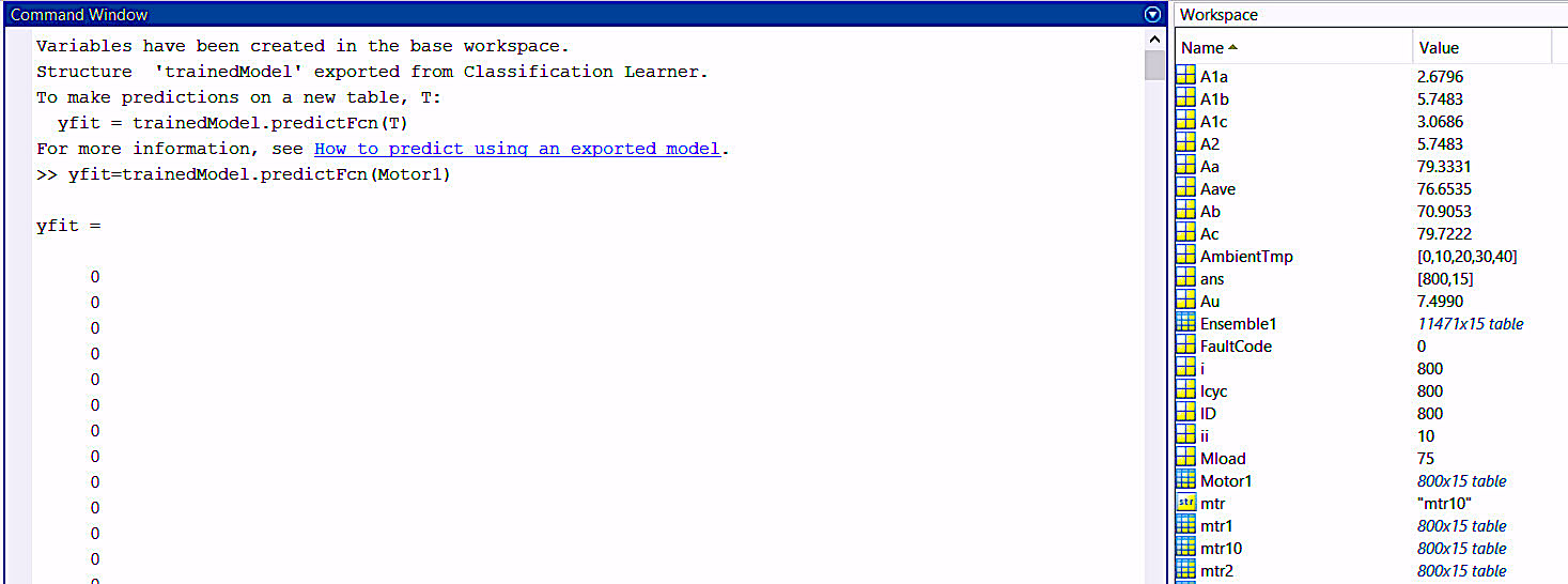
Fig. 8. Testing the trained model with data line by line, from the table “Motor1.”
We have now completed the classification phase of our Machine Learning project and can put it to one side as we explore development of RUL. The RUL process will look at TTFE (Time to Failure Estimation) through several regression options. Those options use some measurement value such as time, operations, distance, among others, along with trends toward defined limits or failure measurements to answer that often asked “how long will it last” question.TRR
SIDEBAR: Sample Code for Creating Comma-Delimited Files in Matlab
For those wishing to explore the method described in this article, Mathworks, provides 30-day trials of its personal and business versions of the Matlab and Simulink systems. The *.csv files created for this article series (as shown in Fig. 1) were developed within Matlab. The resulting code (or script) can be downloaded at the following link:
https://motordoc.com/theramreview-com-machine-learning-article-part-iii-addendum-the-code/
ABOUT THE AUTHOR
Howard Penrose, Ph.D., CMRP, is Founder and President of Motor Doc LLC, Lombard, IL and, among other things, a Past Chair of the Society for Reliability and Maintenance Professionals, Atlanta (smrp.org). Email him at howard@motordoc.com, or info@motordoc.com, and/or visit motordoc.com.
Tags: reliability, availability, maintenance, RAM, electrical systems, electric motors, ML, artificial intelligence, AI, Electrical Signature Analysis, ESA, Motor Current Signature Analysis, MCSA, predictive maintenance, PdM, preventive maintenance, PM, Matlab, mathworks.com, python.org