Evaluation and pre-processing of data is one of the more time-consuming steps in development of a machine-learning (ML) project. In this step, the data scientist views and manipulates the collected data to see what types of artifacts and patterns emerge, including ways and means to clean it up. For the hypothetical motor with which we are working, our selection of Matlab’s software tools give us several capabilities that ease the task of data evaluation and pre-processing.
Click The Following Links To Read Previous Articles In This Series
Part I (Aug. 8, 2021)
In starting our ML project, we first want to see what our data looks like in Excel and how it would appear graphically to identify outliers and noise, as well as help determine the approach we take. Figure 1 shows a portion of an Excel spreadsheet we created in Part III of this article series (see link below).
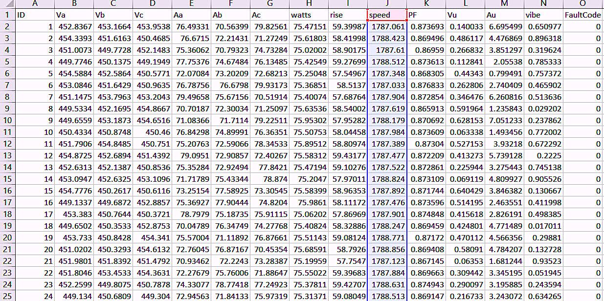
Fig. 1. An Excel spreadsheet view of the data table we generated in Part III of this article series.
We then group the data to see what the system looks like. The noise and outliers can come from data-collection errors and artifacts, general noise in the system, operation of the equipment, and other naturally occurring noise. As shown in Figs. 2 through 6 below, the raw data can be quite noisy.
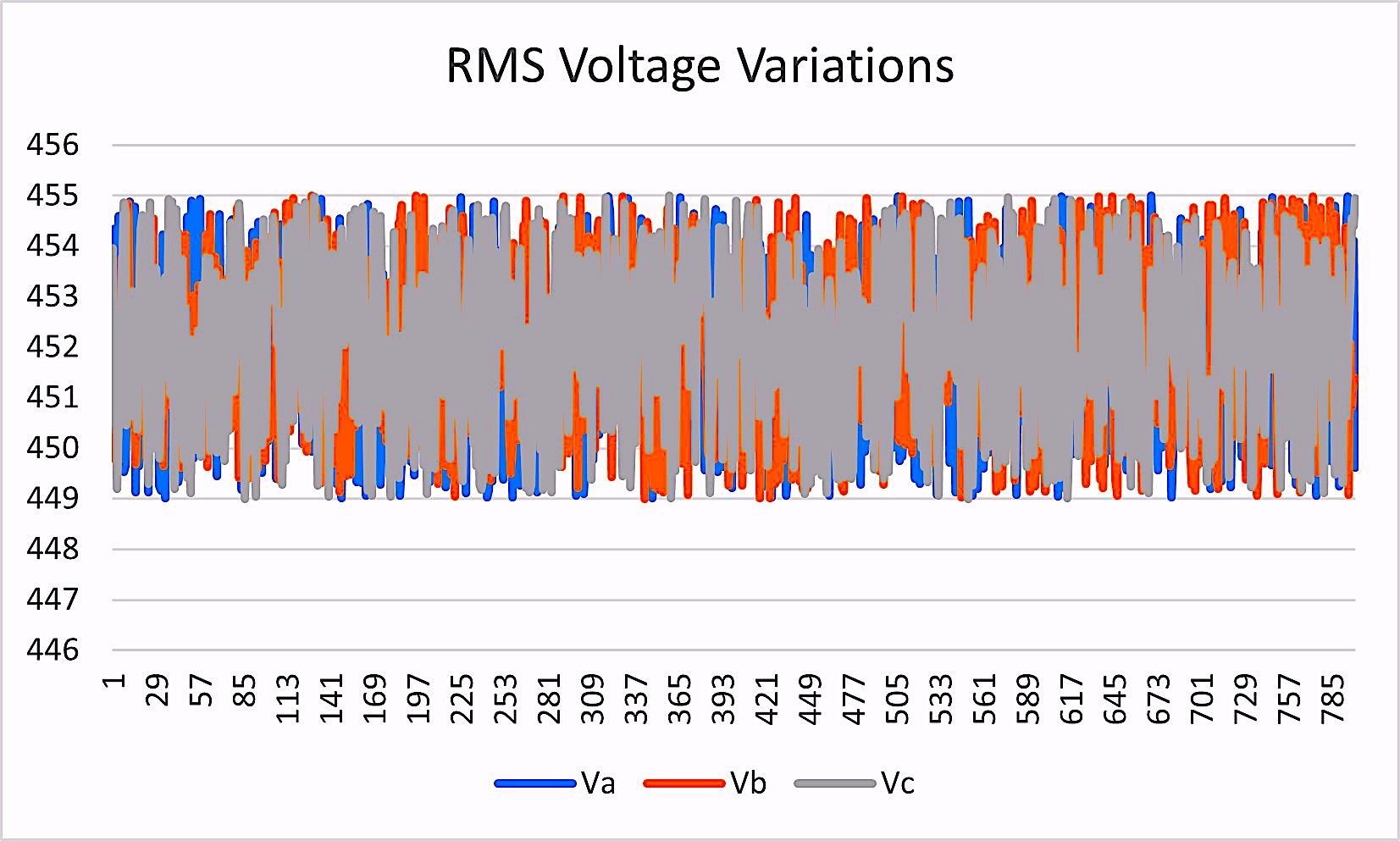
Fig. 2. Raw RMS-voltage-variation data collected hourly.
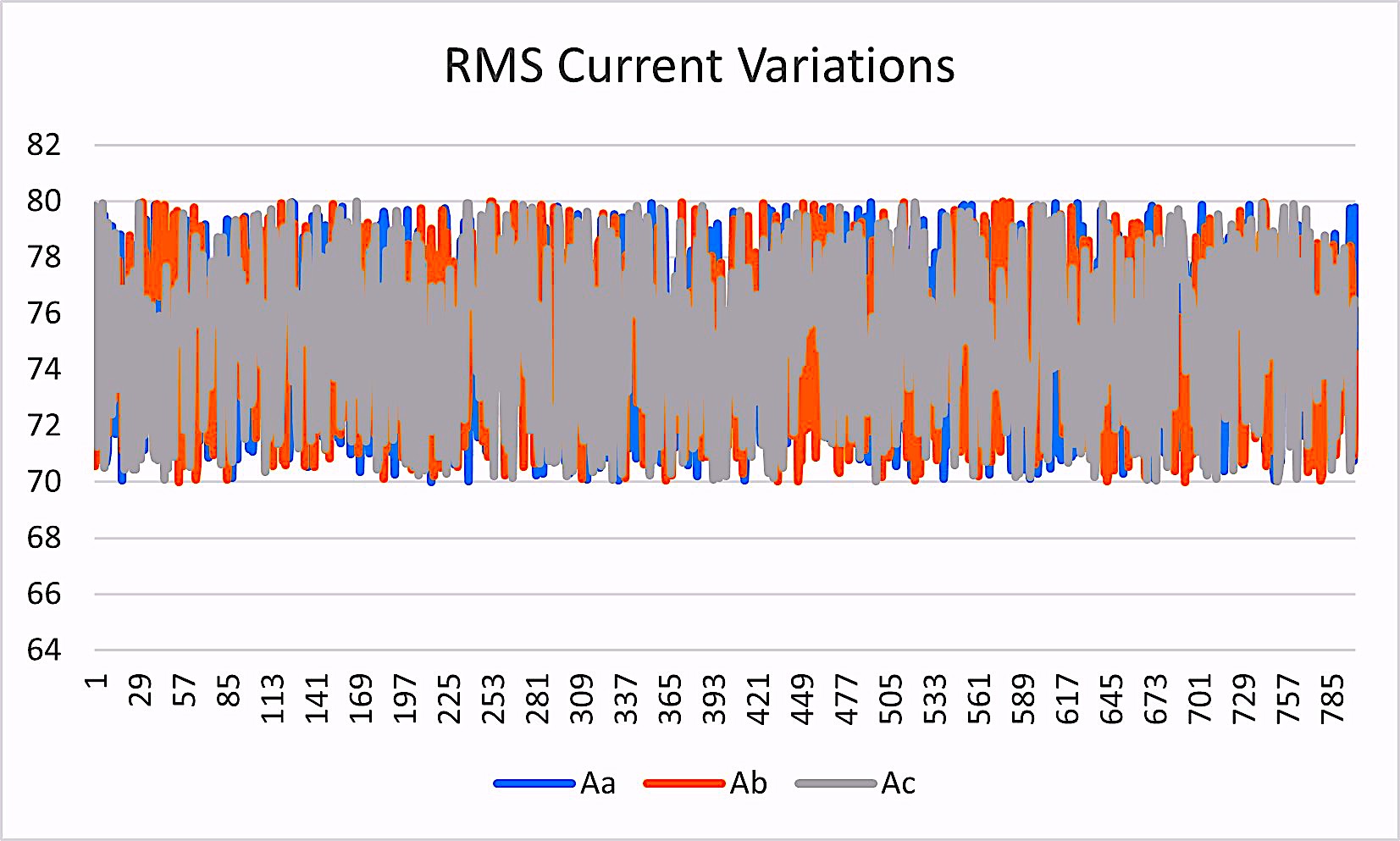
Fig. 3. Raw RMS-current-variation data collected hourly.
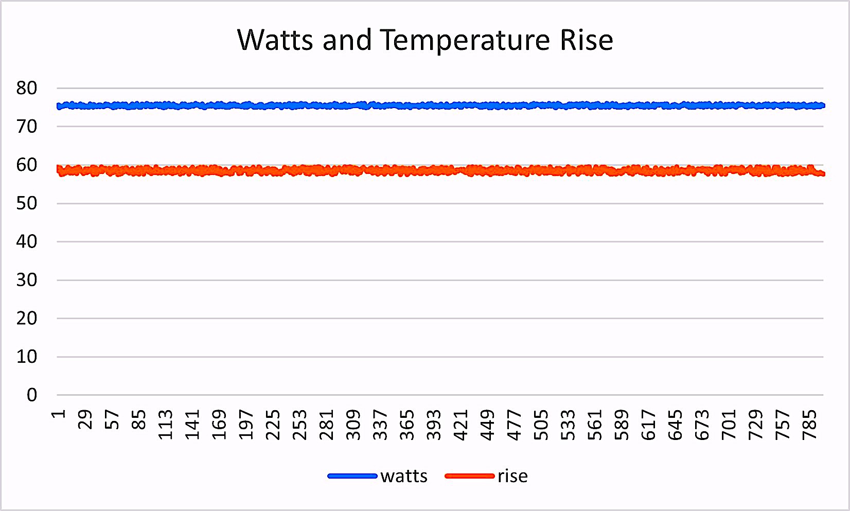
Fig. 4. Raw watts and temperature-rise data collected hourly.
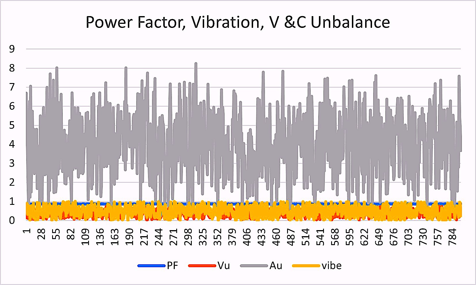
Fig. 5. Raw power-factor, vibration, voltage, and current-unbalance data collected hourly.
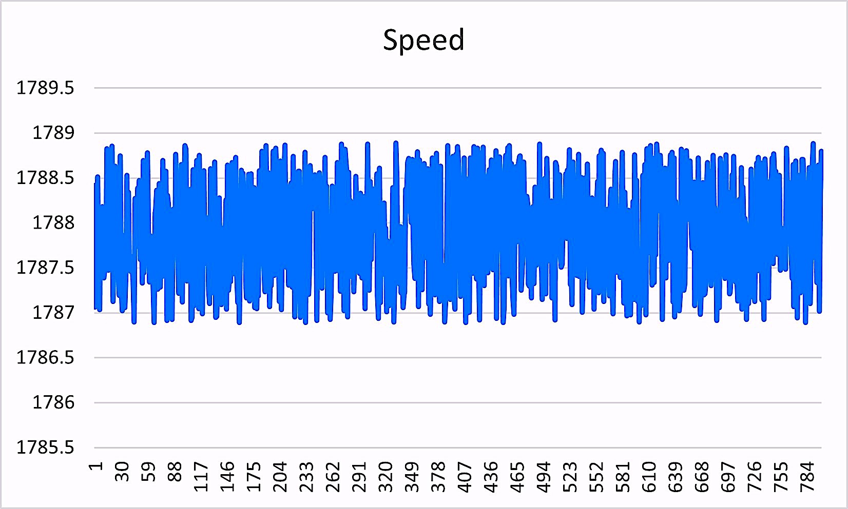
Fig. 6. Raw running-speed-variation data captured hourly.
At this point, our options are 1) to keep the data as is and set our limits and ML training with bands around expected noise; or 2) filter out the data noise using one of several methods.
Because we’re working with raw periodic data and not a high sampling rate, we will use a “smoothing” command and experiment with different filtering methods. These methods range from regression to complex polynomial-filtering algorithms and a variety of “settings” that include the “window” (range of sets of data used to process). With languages such as Python and R, this can be time quite time-consuming for the novice. With Matlab, the process can move somewhat faster, and experimentation can be documented more easily. First, we must import the data as shown in Fig. 7.
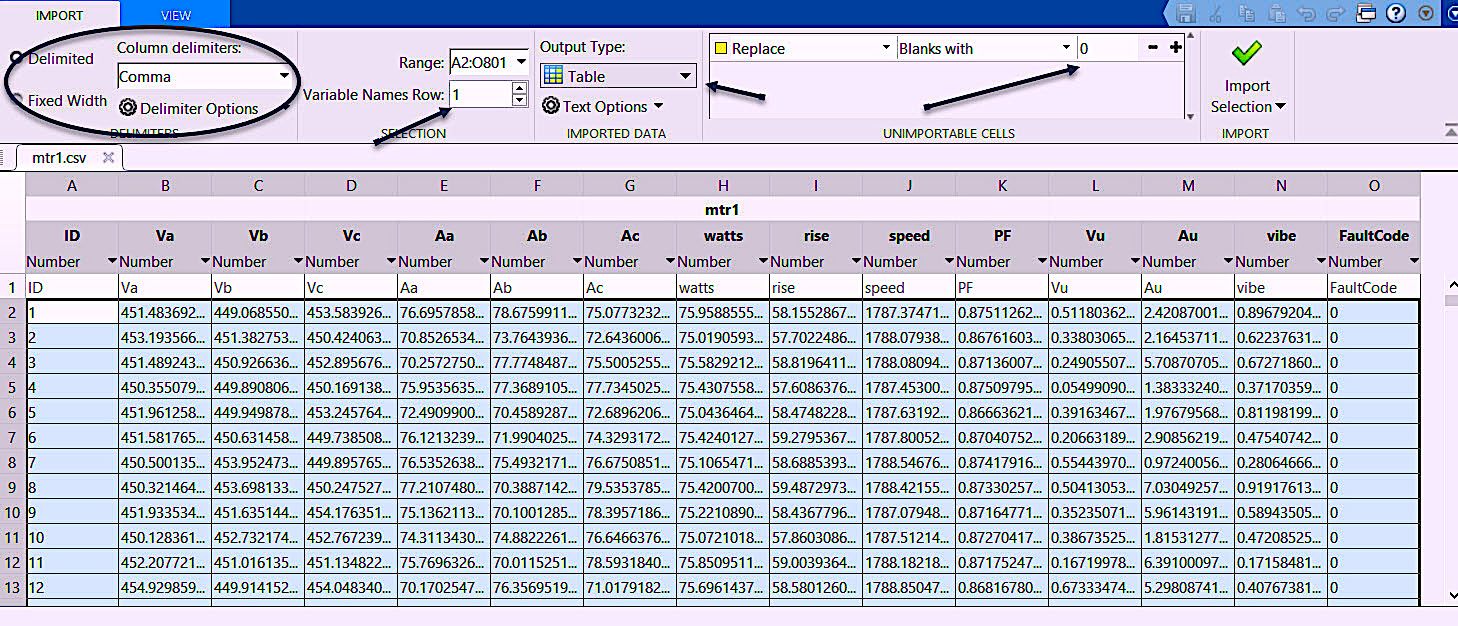
Fig. 7. Matlab’s data-import app or wizard. Select the delimination,
if the variables are present, modify type, etc., determine output and how to manage missing data.
Matlab’s import wizard function (app) provides a graphical interface for determining how imported data will be handled. When all settings are complete, you can opt to 1) have a script or function created using all your settings as part of your final software package; or 2) automate the import process. You then click the check mark ‘Import Selection’ and the data is brought into the workspace for pre-processing.

Fig. 8. Pre-processing by smoothing the data.
In our first pre-processing iterations, (Fig. 8), we determined the best method was to smooth the data. In developing this week’s article, we experimented with multiple filtering methods before selecting a “movmedian” method and a window of “20” (meaning 10 before and after the point being smoothed) that cleaned up rapid changes and small outliers in our data. This method is especially helpful with significant outliers, which are random points that may be substantially different from the surrounding points. By selecting a reasonable window, the data looks like Fig. 9 and Fig. 10, which allows us to identify early changes to the data and trend them.
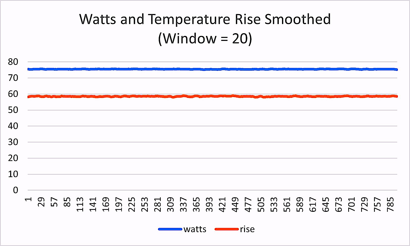
Fig. 9. The same data presented in Fig. 4 after smoothing.
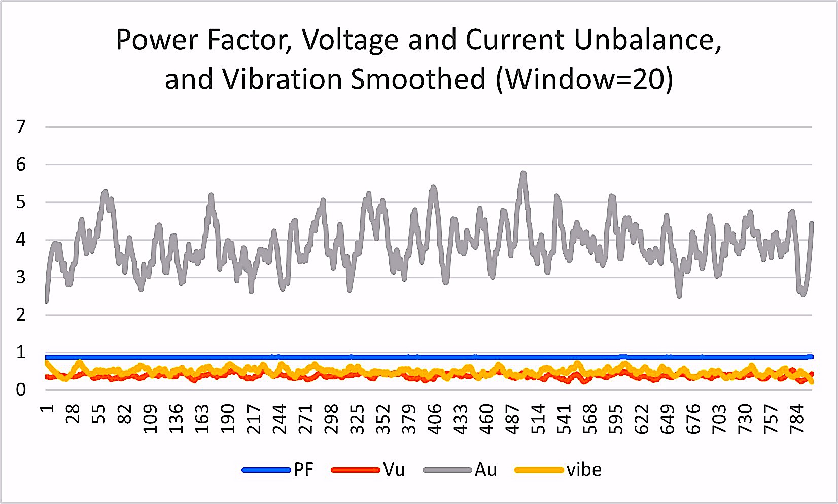
Fig. 10. The same data presented in Fig. 5 after smoothing.
Pre-processing can include other functions and options to manipulate the data into useful information. These functions/options can include the calculation of different features; the selection of specific features for fault analysis; and more.
In the case of our hypothetical electric motor, we’re simply smoothing the data we have to set-up the next step in our machine learning project. This process will also be applied to data collected from the electric motor once we apply the ML software in the real world. We also must generate failure-training data or determine if we are going to create our ML model without failure data. For our purposes, we will generate the failure data using the code we developed in Part III.
In Part V, we’ll discuss how to evaluate and select combined data identified as “good motor” and data representing fault codes for machine learning model. We’ll also include a few tricks to help with early fault detection.TRR
ABOUT THE AUTHOR
Howard Penrose, Ph.D., CMRP, is Founder and President of Motor Doc LLC, Lombard, IL and, among other things, a Past Chair of the Society for Reliability and Maintenance Professionals, Atlanta (smrp.org). Email him at howard@motordoc.com, or info@motordoc.com, and/or visit motordoc.com.
Tags: reliability, availability, maintenance, RAM, electrical systems, electric motors, generators, machine learning, ML, artificial intelligence, AI, Electrical Signature Analysis, ESA, Motor Signature Current Analysis, MCSA, predictive maintenance, PdM, preventive maintenance, PM, Matlab, mathworks.com, python.org