In the first part of this article series (Aug. 8, 2021, see link below), we identified an electric motor and raw data that’s available for performing a Machine Learning (ML) project. We also reviewed the basic steps in the development of an ML system using that same raw data. For purposes of this particular article’s discussion, we will assume the use of our own servers with Matlab and Python engines (code compilers) and libraries (code and function snippets).
Click Here To Read Part I Of This Series (Aug. 8, 2021)
PRELIMINARY DECISIONS
The Matlab system requires licensing for selections of design capabilities, such as predictive-maintenance (PdM) and ML tools. Those licensed offerings include a series of pre-made applications and software code for the development of training, curve fitting, classification, Time-to-Failure Estimation (TTFE, also referred to as Remaining Useful Life [RUL] in the ML community), and other software tools for development of ML programs. Although this approach can be quick and provides a great deal of support, the downside is that licensing for the different capabilities can be cost-prohibitive.
Click here to learn more about Matlab, or go to mathworks.com
Python is an open-source software language for a variety of systems, with Versions 3 and beyond providing ML and and AI (Artificial Intelligence) capabilities (the latest Version is 3.9). All of Python’s capabilities come from a variety of free or low-cost program editors and large libraries of open-source functions. Using Python can be somewhat more time-consuming than working with Matlab, which is a trade-off in terms of cost. However, just like Matlab, there are plenty of books, videos and instructions for the use of Python. Another benefit is that after the 2019 editions of Matlab, many of the functions and code snippets can be used by either program.
Click here to learn more about Python, or go to python.org
The first thing we want to do is start looking at the available data and how it can be mapped out. This can be performed using curve-fitting tools (to develop formulae for curves associated with multiple points, such as what’s shown in Fig. 1). While we will be using the Matlab system for this part, it is understood that similar tools can be used within Python.
Note, when looking at our raw electric motor data, we will only want to use visual tools that make sense (some may not). As an example, for curve fitting, the key is to ensure that you have a reference point, such as ambient temperature for operating temperature and the relationship to temperature rise. In other cases, we would want to reference speed in relation to load or, in the case of variable speed drives (VSDs), to other operating conditions, such as temperature, load, and/or driven equipment conditions.
As shown in Fig. 1, at about 55% load (55kW), the temperature begins to curl up again, which is not representative of real information. This can be eliminated through selection of additional points, or be used within the range that was selected. Another option would be to use some other curve that doesn’t meet all the points can be used. Those decisions are where the designer’s experience and preferences come into play. For instance, using the formula and applying the load (X), you can determine the operating rise (Y), which is the temperature above the ambient temperature at which the motor is designed to operate. If we don’t have operating or failure data, this would be the type of data that we would need to use.
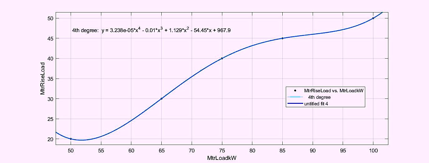
Fig. 1. Curve fitting for motor load versus temperature rise.
The different views in Fig. 2 and Fig. 3 provide some context for the data and what it will mean. They also allow us to develop training data for the algorithms with which we will begin working. At the same time, manual manipulation of the data is important to ensure there’s something meaningful in the information that we have chosen to use and how it relates to what we are trying to do.
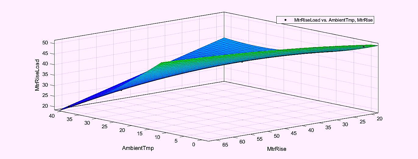
Fig. 2. Load versus ambient temperature versus motor temperature rise.
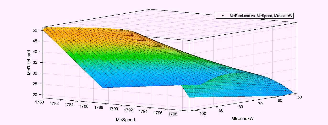
Fig. 3. Speed versus load versus temperature.
COMING UP
The next article in this series (Part 3), will discuss development of test and training data to create a classification model and degradation models for RUL calculation. These types of models, especially when no real data is at hand, can be upgraded later with operating information and failure data. Until that type of information is available, though, there are several other options. We will also explore them in this series.TRR
ABOUT THE AUTHOR
Howard Penrose, Ph.D., CMRP, is Founder and President of Motor Doc LLC, Lombard, IL and, among other things, a Past Chair of the Society for Reliability and Maintenance Professionals, Atlanta (smrp.org). Email him at howard@motordoc.com, or info@motordoc.com, and/or visit motordoc.com.
Tags: reliability, availability, maintenance, RAM, electrical systems, electric motors, generators, machine learning, ML, artificial intelligence, AI, Electrical Signature Analysis, ESA, Motor Signature Current Analysis, MCSA, predictive maintenance, PdM, preventive maintenance, PM, Matlab, mathworks.com, python.org