
In Part III of this article series (Nov. 20, 2021, see link below), we discussed common and linear-type failure modes from mechanical systems as represented in the P-F curve. Mechanical equipment fails in terms of a “natural log” hazard curve, wherein the resistance to failure decreases or the possibility of failure increases, as time or cycles progress to the point of functional failure. In this article, we’ll discuss the more prevalent failure modes that occur with dielectric systems, such as electric-motor insulation, cable-insulation, and transformer-insulation systems.
The types of hazard curves associated with dielectrics are often thought of as “instantaneous,” because they don’t fit typical expectations and assumptions associated with mechanical wear and. As a result, they become an anomaly to reliability practitioners. (Note: Other systems fall within the realm of non-linear hazard and failure curves. They’ll be identified as this series continues.)
Those involved with dielectric systems, such as electric machinery, power insulation systems, and even electronics, understand that common degradation is a function of temperature applied to both an operating circuit and a circuit at rest. This means when we’re reviewing the aging of an electrical device that we must consider degradation occurring when the system is undergoing operational stresses, as well as aging of the system as it sits idle. The first step, however, is understanding the aging system due to temperature, which is a function of the Arrhenius equation, as applied to electrical insulation (Equation 1).
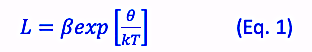
Where L is the expected life of the insulation system in terms of time; ß is an experimental constant associated with the material(s); ϴ is the activation energy in units of eV (electron volts); k is the Boltzmann Constant (0.8617 x 10⁻⁴eV/T; and T is the absolute temperature of the insulation system in Kelvin.
What’s particularly interesting about Equation 1 is that with modern electrical-insulation systems, L will often be measured in near-infinite time. That’s a far cry from the 20 years for small motors and 40 years for medium and high voltage motors that we associate with insulation system life.
After the 1960s, insulation-system chemistry made significant advances. In the 1990s, industry standards caught up and included, in 1991 (inactive-withdrawn in 1997) IEEE Std 1064, “IEEE Guide for Multifactor Stress Functional Testing of Electrical Insulation Systems.” The approach has been to evaluate the endurance of the insulation system through a variety of testing methodologies which have expanded due to the types of electrical environments that the systems have been exposed to. In addition, the mix of different insulation systems and material transitions have a direct impact on the capability of the insulation system across an expected insulation life.
So, how does all this impact our ability to review Remaining Useful Life (RUL) or Time to Failure Estimation (TTFE) of an electric machine, cable, or transformer? If we listen to traditional wisdom and try to predict exact life, then we would come to believe it is impossible. If, however, we consider the issue from an TTFE standpoint, we can review probable life, as we begin to understand the application, environment, operating context, and conditions surrounding the stresses associated with the machine.
For analysis of insulation systems, we need a baseline. We start with the base thermal stress shown in Equation 2.
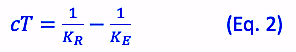
Where cT is base thermal stress: KE is the absolute temperature; and KR is absolute room temperature at 298 Kelvin.
The formulae for base thermal life (Equation 3) and base thermal life at room temperature (Equation 4) are shown below.
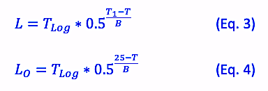
Where TLog is in hours; T1 is the temperature of interest; and T is the thermal life of the thermal life study of the material all in degrees Centigrade (C).
The thermo-electro stress (LSO) is applied through the insulation-system voltage stress formula, shown in Equation 5.
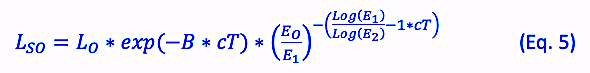
Where EO is voltage applied to the winding; E1 is the voltage applied during life studies; and E2 is the published electrical endurance of the winding insulation system.
Equation 5 provides the baseline for the insulation-system life. In keeping with concerns over temperature, the next consideration is thermal shock (Equation 6). Thermal shock is the result of rapid heating and cooling of insulation systems that can be driven by starts, ambient temperature, and length of start times.
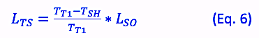
Where LTS is the expected life of the system based on the amount of time within the thermal-shock value at 10 C from literature; and TT1 is the log average life from thermal shock testing also from the literature.
This, in turn, raises the issue of machine vibration, which due to its impact on insulation life, must be taken into account (Equation. 7). The level and type of vibration must be considered from testing or averages.
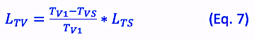
Where LTV is the expected life in hours; TVS is the severe vibration value; and TV1 is the log life average from testing.
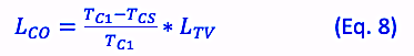
While there are additional conditions to consider, the final major condition for the purpose of this article, is contamination (Equation. 8). As with Equations 6 and 7, contamination life (LCO) is based upon contamination exposure time (TCS) and log average life by experiment (TC1).
From a manufacturer’s perspective, this approach can be utilized to work along with determining the point at which a percentage of machines would fail. Experimentation is required to provide accurate data analysis of this type. However, some information can be considered and calculated in a way to project life, and then be followed up with data collection to determine how quickly the system is degrading.
In Part V, we will look at a case study associated with the methodology from this article using a 50-hp electric motor operating across-the-line.TRR
Click The Following Links For Parts I And II Of This Short Series
“Part I, The Possibilities Of Probability: In Reliability And Predictive Maintenance” (Nov. 6, 2021)
“Part II, The Possibilities Of Probability: In MTBF” (Nov. 15, 2021)
“Part III, The Possibilities Of Probability: In Failure Curves And RUL” (Nov. 20, 2021)
ABOUT THE AUTHOR
Howard Penrose, Ph.D., CMRP, is Founder and President of Motor Doc LLC, Lombard, IL and, among other things, a Past Chair of the Society for Maintenance and Reliability Professionals, Atlanta (smrp.org). Email him at howard@motordoc.com, or info@motordoc.com, and/or visit motordoc.com.
Tags: reliability, availability, maintenance, RAM, electrical systems, predictive maintenance, Artificial/Augmented Intelligence, AI, Machine Learning (ML), Internet of Things, IoT, P-F Curve