
One of the most powerful and straightforward measurements of equipment reliability is Mean Time Between Failure (MTBF), which lets the reliability engineer roughly estimate conditions surrounding a system. Some will criticize the use of MTBF as a reliability tool while overlooking the fact that, as a lagging indicator, it sets the basis for industrial- and reliability-engineering improvement opportunities (refer to Drew Troyer’s recent articles on MTBF/MTTR in the links below). For example, to identify an area of a plant for investigation, equipment or systems that have poor MTBF will stand out, regardless of the cause. This means that opportunities can be rapidly identified without conducting in-depth research on every system in advance.
MTBF provides the basis for other functions used to sketch out conditions for a system or facility. These include Mean Time To Repair (MTTR); Mean Time To Failure (MTTF), Time To Failure Estimation (TTFE), Failure Rate (λ), and the Reliability Function (R). These functions are also relatively simple to figure out and only require that the same time measurement be used when comparing:
- MTBF: Number of Failures/Time Period
- MTTR: Time to Repair/Number of Failures
- MTTF: (Time of Detection – Time Failed)/Number of Failures
- Failure Rate: 1/MTBF
- Reliability Function: R = e–tλ where t is the time of interest
- TTFE = 1-R at the time of interest (probability that the equipment will survive to the time of interest).
The Reliability Function can be used at the component or sub-system level and applied across a system to look at series or parallel components of the system, each with their own conditions.
The TTFE of a fault can then be evaluated by component, by reviewing the time since the last failure of each sub-system, or across the system assuming a start from time “0.”
The series Failure rate (FS) is simply performed by multiplying each R by each component in the system, such as FS = (R1)(R2)…(Rn). The parallel failure rate (FP) is found as FP = (R1 + R2) – (R1)(R2) for two systems in parallel, and FP = 1 – (1 – F)n for three or more identical systems in parallel.
Since we already know that we’re looking at probabilities, let’s use an MTBF-related example of a hypothetical parallel pump system and see where we need to expend some resources. Our hypothetical system has one source of incoming power; one variable frequency drive (VFD); two electric motors; two couplings; two pumps; and two valves. After determining that we will look at the system by hours of operation (6000/year), the equipment’s history provided the information in Table I.
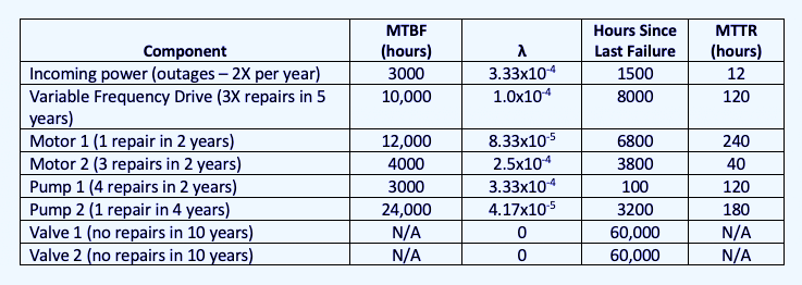
Table I: Failure Rates of a hypothetical parallel pump system.
For determining the present availability of these systems and components, we would first evaluate the motor and pump in series; then each motor and pump system in parallel; then the incoming power, VFD, and motor/pump systems in series. By doing so, we can quickly see the weakest points in the system (incoming power) and other problems that stand out, such as Motor 2 and Pump 1, that would require further investigation. Plugging those numbers into the formulae gives us Table II. For example, the Reliability Function applied to incoming power would be:
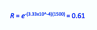
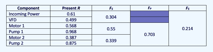
Table II. Evaluation of hypothetical parallel-pump-system components.
While we don’t know the exact time between the Motor 2 and Pump 1 failures, the overall picture provides a good idea as to which systems and components should be addressed, and a review of those specific items can be conducted. Note: As neither valve has failed, no failure rate is available. However, a strategy for how to maintain or monitor the valves can be determined.
It is also important to note that we have two single points of failure and the one with the highest potential for failure involves the loss of power. Knowing the time to repair the conditions involved in system failures also provides the means to determine the impact and associated downtime costs that provide the information necessary to justify corrective actions.
The information in Tables I and II can also be used to forecast availability by adding the time of interest to the time since the last failures. This approach can be used with a spreadsheet or software to calculate TTFE. Beyond the functions around MTBF, more advanced evaluation of reliability probability can be determined for systems that are selected for in-depth analysis.
COMING UP
Next week, in Part III of this short series, we will discuss probability related to failure curves, such as wearout, bathtub, and linear, including when and where they exist. This discussion will set the basis for additional ones around failure definition, remaining useful life, and Time to Failure Estimation.TRR
Click The Following Links To Read The Referenced Drew Troyer Articles
“Lagging Indicators For Asset Management: MTBF/MTTF, Part 1” (Aug. 15, 2021)
“Lagging Indicators For Asset Management: MTBF/MTTR, Part 2” (Aug. 23, 2021)
ABOUT THE AUTHOR
Howard Penrose, Ph.D., CMRP, is Founder and President of Motor Doc LLC, Lombard, IL and, among other things, a Past Chair of the Society for Reliability and Maintenance Professionals, Atlanta (smrp.org). Email him at howard@motordoc.com, or info@motordoc.com, and/or visit motordoc.com.
Tags: reliability, availability, maintenance, RAM, electrical systems, Mean Time Between Failure, MTBF