
In Part 1 of this 3-part article (May 8, 2022, see link below), we discussed taking a raw data sample and using a simple data-processing technique to make it look like something we might see on a Motor Current Signature Analyzer or Electrical Signal Analyzer (MCSA and ESA, respectively). In this part, we’re starting where we left off: We’re making the data look sharper with windows and converting the y-axis of the spectra into dB that can be used to determine severity and condition.
Click Here To Read Part 1 Of This Article
As explained in Part 1, the dataset we’re using for a rudimentary transformation to a spectral analysis was taken at 10kHz per channel across 10 seconds on a 10-hp, 1,175-rpm, 14.3 Amp electric motor. Since we are using Python and the SciPy FFT library, there may be a few shortcomings, but we will be able to analyze this data in the end.
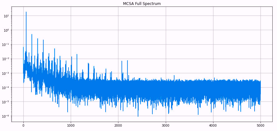 Fig. 1. The FFT of the processed data from Part 1.
No windowing has been performed.
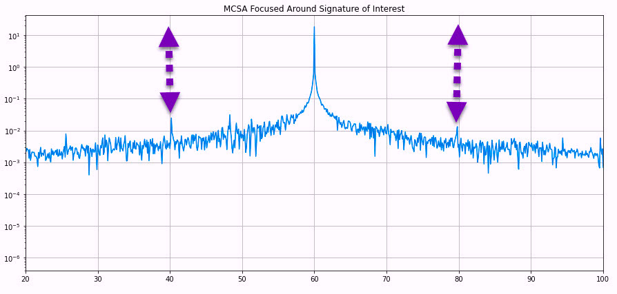 Fig. 2. Original preprocessed raw data showing running-speed
sidebands in log format (y-axis).
As noted in Fig. 1 and Fig. 2, there are what appear to be +/- running-speed peak sidebands at 40 Hz and 80 Hz around line frequency. However, the values are not such that we can properly evaluate them down from the peaks as identified in the Fig. 2 arrows. The common method we use for evaluating a voltage or current signature is in dB down from the peak value at the line frequency.
THE PROCESS
One of the first things we need to do is sharpen the peaks and flesh out any additional signals. For this, we need to smooth the data. This is performed through ‘windowing:’
♦ Hanning Window uses the shaped cosine wave with 1 added so that it is positive. The sampled signal is multiplied by the Hanning Function, which also forces the ends of the data sample to zero. It’s important to note that the Hanning Window is used with continuous signals as interrupted conditions will remove the remaining portion of the waveshape. This will result in sharper peaks.
♦ Flat Top Window, also a smoothing function, is wider and smoother than the Hanning Window, but the amplitude accuracy is far better. While the example in this article is of a simple 60Hz clean signal, any filter will perform well. A Flat Top Window, however, performs best in VFD applications or those with high harmonics.
♦ Hamming Window is an improved form of the Hanning Window using 25/46 instead of ‘1’ that allows some negative values. Results in sharp peaks and frequency accuracy.
 Fig. 3. The 5kHz spectra following Hanning Window application.
When we perform the Hanning (Hann) Window, the spectral data appears as shown in Figure 3. At 5kHz on the x-axis, the difference is not as noticeable as that between Fig. 2 and Fig. 4.
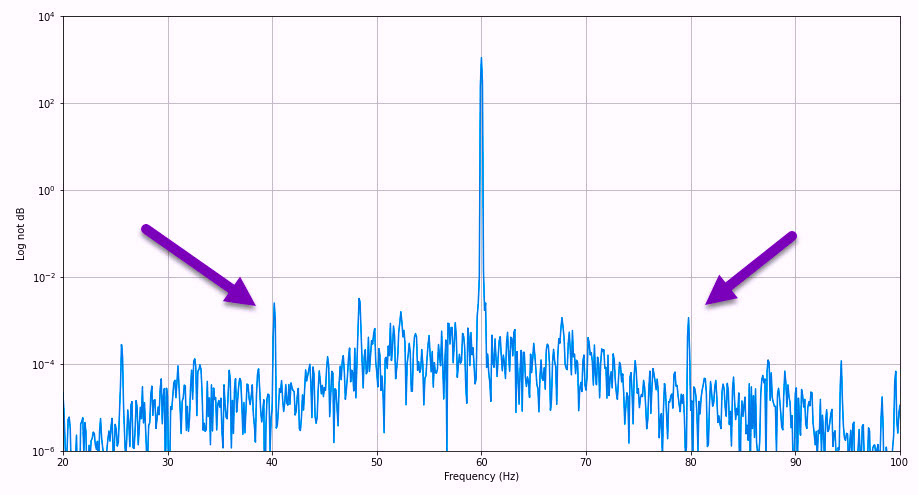 Fig. 4. Hanning Window on raw data: Note peaks at 40 Hz and 80Hz,
which are the running speeds.
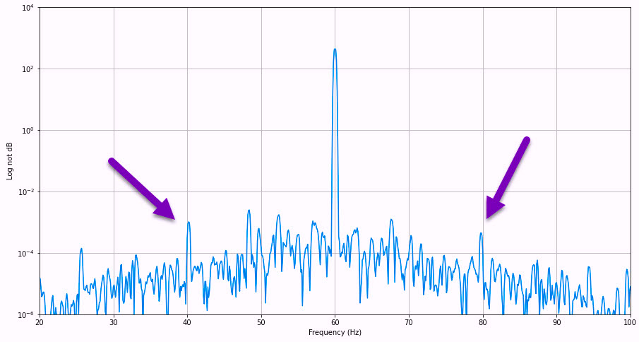 Fig. 5. Flat Top Window: Note that peaks seem more rounded
than in Hanning or Hamming Windows.
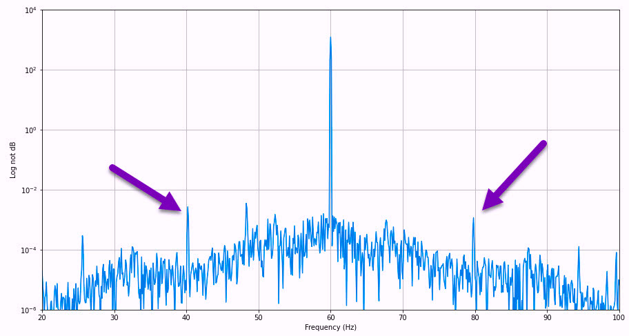 Fig. 6. Hamming Window: Note that the peaks are once again sharp,
and peak values appear to be similar to those in Fig. 4.
As noted, in the Flat Top Window, the peaks are rounded and not as sharp as in Fig. 4 and Fig. 6. The next step would be to introduce a dB value on the Y-axis. Once that’s done, the values can then be counted “down” to each peak of interest from the line frequency peak.
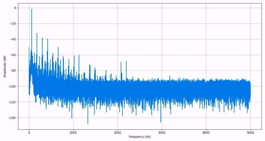 Fig. 7. Current spectra of one phase in -dB.
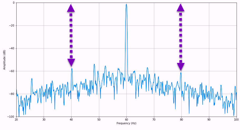 Fig. 8. Low-frequency spectrum showing running speed peaks at -57 dB.
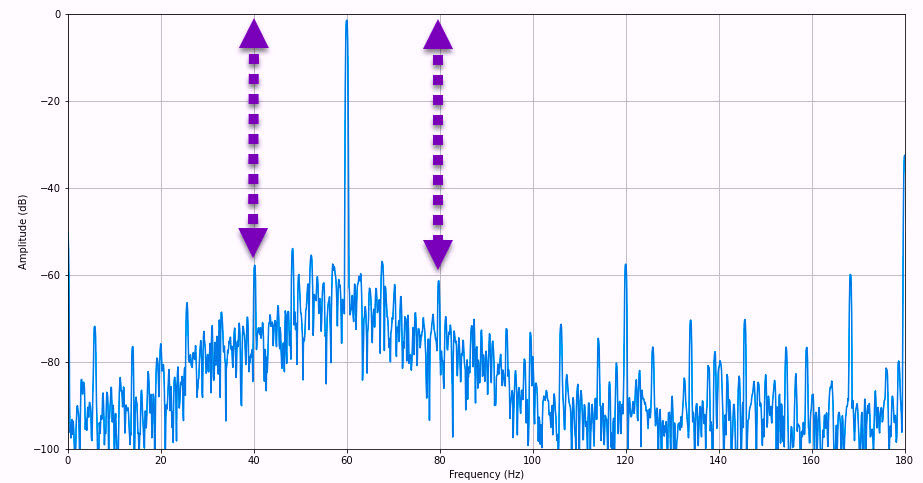
Fig. 9. Peaks on 180Hz spectrum.
As can be seen in Fig. 8 and Fig. 9, the running-speed peaks do exist. There is a possibility of some type of low-level pole pass frequency, but the amount of noise still present is masking issues outside of ones that have resulted in high peaks.
COMING UP
In Part 3, we’ll further clean up data with a larger dataset from an instrument that takes 12,000 samples per second over 48 seconds, including averages, and a few other tricks. We’ll also consider how to identify peaks of interest.TRR
ABOUT THE AUTHOR
Howard Penrose, Ph.D., CMRP, is Founder and President of Motor Doc LLC, Lombard, IL and, among other things, a Past Chair of the Society for Maintenance and Reliability Professionals, Atlanta (smrp.org). Email him at howard@motordoc.com, or info@motordoc.com, and/or visit motordoc.com.
Tags: reliability, availability, maintenance, RAM, asset management, electric motors, Motor Current Signature Analysis, MCSA, Electrical Signature Analysis, ESA, vibration analysis, motor testing