Over the past few months in The RAM Review, we’ve been waxing philosophically on large-scale electrical issues. Now, let us dive past the basics and get more specific. In particular, let’s get into the programming nitty-gritty of Motor Current Signature Analysis (MCSA) and Electrical Signature Analysis (ESA), vibration analysis, and any other technologies that convert data to spectra for evaluation.
The purpose of this discussion is to provide an idea of what and why things are done within spectral and IIoT analysis of data. We’ll be exploring a truly rudimentary evaluation of a dataset on a 10-hp, 1175 rpm, 14.3 Amp, electric motor tested with a raw-data collector (not a commercial analyzer) at 10kHz sampling across 10 seconds. While not particularly accurate, the technology is good enough for our purposes. Note that we are using Python and the SciPy FFT library as we walk through this multi-part adventure. In the end, we will have demonstrated the importance of data processing, data resolution, filters, and why different instruments are effective at different loads of the motors under test, as well as why one instrument takes close to 10 minutes to collect data, while another takes less than a minute.
At 10 seconds and 10kHz per channel, the data provided in a csv file is 100,000 rows of three phases of voltage and three phases of current. The provided data is not time-stamped (Fig. 1), but for the purposes of this multi-part article, we will work through things programmatically.
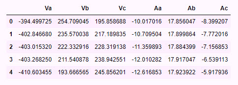
Fig. 1. The first five rows from the dataset we are using in this article’s example.
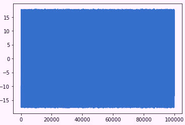
Fig. 2. All data from one phase of current. The X-axis is the number of datasets.
The Y-axis is the peak-to-peak current.
In Fig. 2, we present all of our data at once, and without any processing. This is the peak-to-peak across 10 seconds. While there are no particular conditions noted here, we would be able to see variations and waves if the motor had a significant rotor bar issue or other severe condition.
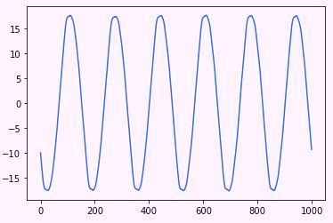
Fig. 3. A selection of Fig. 2 data across 1/10th of a second, or 1,000 data points.
Figure 3 is a snapshot of the data from Fig. 2. The waveform appears almost perfect, so can there be defects in this motor? One of the reasons we use spectral analysis is to pull out the very small values in this type of data. What happens if we process this data raw through an FFT (Fast Fourier Transform)?
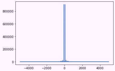
Fig. 4. The X-axis is frequency, and the Y-axis is unknown.
As noted in Fig. 4, if the data is simply processed raw, the results are interesting using the Python tools, and are similar using MatLab. Leaving out the extreme Y-axis values, why do we have both positive and negative frequencies? It’s due to the nature of the amplitude-modulated data that we are analyzing, which will cause multiple sideband peaks, and also because about half the numbers have a negative value (see Fig. 1). This is managed by some basic processing using absolute values. In the end we have Fig. 5, in which we have up to 5 kHz on the X-axis. However, because of the amount of noise present using this raw data, we have limited it to 500Hz. As you can see, we already have a peak at 60Hz and sidebands around it. At the same time, we’re still dealing with some interesting Y-axis values.
Note: if we had worked with this as time-series data, there would be more control over the Y-axis values, which would appear as ~16 Amps peak at 60Hz. Without the time stamping, however, the libraries we are using basically manipulate the information and produce odd numbers.
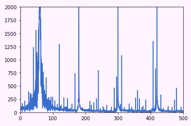
Figure 5: X-axis is frequency, limited to 500 Hz. The Y-axis is an unknown value.
We know that use of data such as that shown in Fig. 5, even if the Y-axis was producing correct values, would not give us a good reference. This information is known as “linear” data. However, we do know that we have information that can be processed. For the purposes of this article (Part 1), we will process the spectrum using the commands to select the Nyquist (1/2 of the sampling rate for ESA/MCSA). Then, in processing a spectra in dB (Decibels), we’ll use the 10*log10 of the peaks (used for voltage) instead of the 20*log10 (used for current).
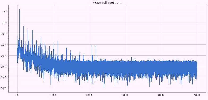
Fig. 6. The X-axis is frequency (Hz); the Y-axis is dB (Decibels)
counting down from the peak current.
Referring to Fig. 6, note that the spectra look more like what we would expect to see in an MCSA-data screen. While there’s still plenty do to provide values on the Y-axis to help in an analysis, we are approaching the point where we can get an idea of problems the motor might be having. As shown in Fig. 7, the 1175-rpm motor will turn between (1175RPM/60Hz) 19.58Hz and 20Hz. Two peaks present at 60Hz + ~20Hz and 60Hz – ~20Hz, which would be running speed. This situation would indicate some level of unbalance or misalignment.
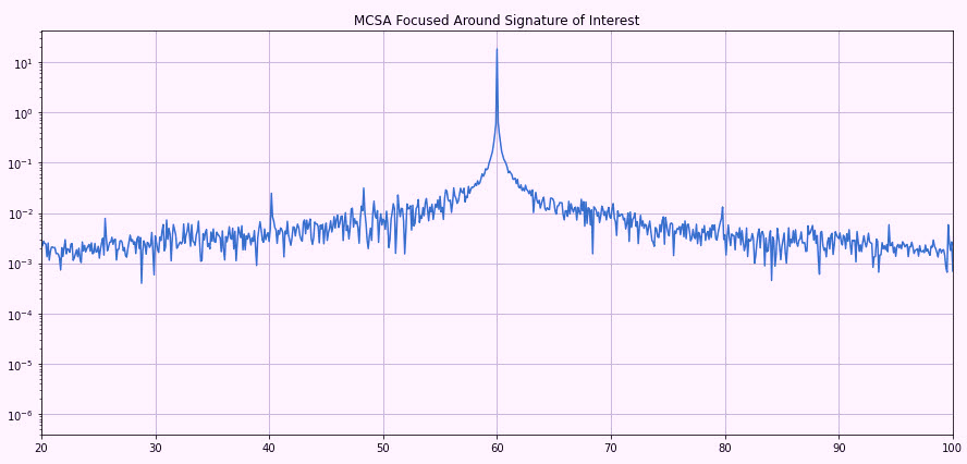
Fig. 7. The X-axis is frequency and Y-axis is in -dB. Note peaks close to
40Hz and 80Hz relating to running speed of the motor.
Our first areas of interest are the peak at 60Hz with a wide base and those that aren’t very sharp. Other conditions may also be present. There are several reasons for this, including: 1) the noise, as we have not filtered it; and 2) the bin-size, or resolution.
With the information that we have (10 seconds of 10,000 samples per second), what do we know about our accuracy? First, the FMAX, which we know is ½ of the sample rate (5kHz). The FFT block size would be part of the equation, which we will have to work with in programming. For this, however, the block size was 9,600, which we then use as 5000Hz/(9600/2) = 1.04-Hz resolution on each peak. This means that peaks such as running speed are accurate to ~60 rpm in our present evaluation. If we can drive that block size up, we have a more accurate number.
We know that our motor is relatively well loaded, so the peaks sitting almost on top of 60Hz +/- 20Hz are not accurate, meaning that we have to be over ~80% load to identify most defects. With the present data, casting voids or broken rotor bars would not be apparent, and high ground noise means that other conditions such as bearings cannot be identified. High-frequency issues, such as static and dynamic eccentricity, which are used to help identify specific defects are also not apparent. Noise can be reduced by increasing averages and applying different types of filter windows, which we will explore with this dataset next week (in Part 2). Well also see if we can take additional steps to identify conditions and be more accurate with our data.
At this point, we’ve seen what we can from a basic set of collected data with some basic processing, which was then converted to rudimentary spectra for analysis. This is much the same way that vibration, ultrasound, and other types of datasets are managed. While we won’t go too far in-depth with regard to software development, we will discuss how different parts of an IoT or data-collector spectral analysis works and what all the tech-speak means.TRR
ABOUT THE AUTHOR
Howard Penrose, Ph.D., CMRP, is Founder and President of Motor Doc LLC, Lombard, IL and, among other things, a Past Chair of the Society for Maintenance and Reliability Professionals, Atlanta (smrp.org). Email him at howard@motordoc.com, or info@motordoc.com, and/or visit motordoc.com.
Tags: reliability, availability, maintenance, RAM, asset management, electric motors, Motor Current Signature Analysis, MCSA, Electrical Signature Analysis, ESA, vibration analysis, motor testing