Over the past six months, I’ve focused on high-level metrics and Key Performance Indicators (KPIs) for asset management. We’ve addressed Mean Time Between/To Failure (MTBF/MTTR), Overall Equipment Effectiveness (OEE) and its associated loss categories, Return on Net Assets (RONA), Economic Value Added (EVA), Balance Sheet Basics, and a host of other KPIs. Going forward, we’ll dive into more operational metrics for Maintenance & Asset Management, Production & Lean Operations, Supply Chain, Environmentally Sustainable Manufacturing, and Safety & Health. But before we start moving in that direction, this week I want to close the topic of strategic and operational asset management KPIs by discussing the income statement.
INCOME STATEMENT: THE NUMERATOR FOR RONA
Readers may recall from my Feb. 14, 2022, article about Return on Net Assets (RONA) (see link below) that, in the very simplest of terms, RONA is the income statement divided by the balance sheet (or the firm’s profit divided by the capital investment divided by that profit). A firm’s income statement reveals it Earnings Before Interest & Tax (EBIT) or Earnings Before Interest, Tax, Depreciation & Amortization (EBITDA). While there are differences between EBIT and EBITDA, they’re not relevant to our discussion linking asset-performance management to the income statement.
The income statement, at its simplest level, reveals profits by subtracting Total Cost from Total Revenue. But there numerous inputs to those figures that are very much the business of Asset Management Professionals. Let’s explore them. Keep your focus on Fig. 1 as we do.
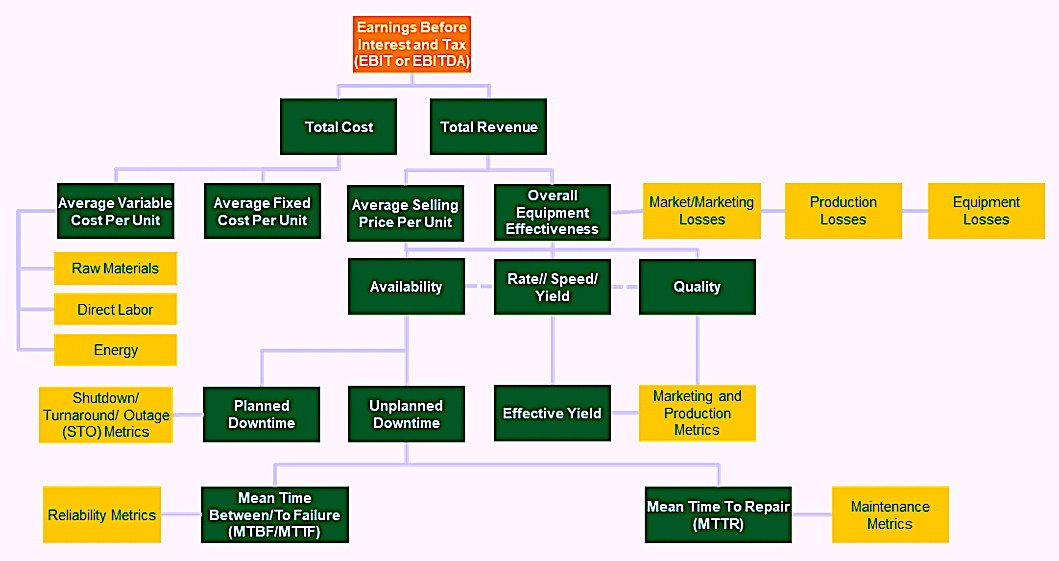
Fig. 1. This diagram links Mean Time Between/To Failure (MTBF/MTTF)
and Mean Time To Repair (MTTR) to profit.
ASSET-MANAGEMENT DRIVERS OF REVENUE
Revenue is calculated by multiplying the total units sold by the average selling price per unit. I previously addressed Overall Equipment Effectiveness (OEE), and associated losses in great detail (see link to access 12 OEE articles below). OEE is the product of multiply Availability, Rate/Speed/Yield, and Quality performance A score of 100% represents perfection, which means that the plant ran 8,760 hours during a year at 100% of it’s highest sustainable rate of production and produced no defective output. It would be great to achieve such production levels, but doing so is a big ask. Most organizations suffer from a variety of Market/Marketing-, Production-, and/or Equipment-induced losses over time. Sometimes those losses are planned and in other instances they are unplanned. It’s our objective as asset managers to eliminate unplanned losses and minimize planned ones. It’s important to note at this point that we seek to optimize OEE (NOT maximize it) to maximize RONA.
Click Here To Access The Author’s 12 Articles On Overall Equipment Effectiveness (OEE)
Asset performance and OEE most directly affect the number of units that are available to sell, but it can also impact the average selling price per unit via the Quality pathway. Poorly operating equipment can produce off-quality product that must be sold at a discount or sold as scrap. If a large percentage of production must be sold as off-grade or scrap, it can substantially reduce the average per-unit selling price. If the plant is producing controlled substances, such as pharmaceutical products, off-quality product may be a total loss of revenue and, in some instances, a cost penalty for disposal of that product.
In a study by The Aberdeen Group, the average Availability across a wide array of industries was found to be 87.2%, and the Average Rate/Speed/Yield was 81.9% (Table I). However, upper quartile performers delivered Availability of 88.8% and Rate/Speed/Yield of 84.2%. These differences may seem small, but they have a huge impact on the bottom line (which we’ll discuss later).
ASSET MANAGEMENT DRIVERS OF COST
Apart from raw materials, energy and direct labor, asset management typically represents the highest cost category for most organizations in the manufacturing, process and other equipment asset-intensive organizations. These costs include parts, tools, labor and materials for routine maintenance and repair and for sustaining capital costs. In their 2009 study, the Aberdeen Group estimated the asset management costs for the average organization as 20.8% of sales – significant by any standard (Table I). By contrast, upper quartile asset managers incurred asset management costs of 17.2% Again, these differences may seem small, but the difference is hugely impactful in terms of profitability.
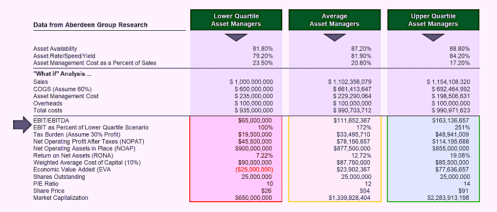
Table I. Profit performance comparison for an imaginary company assuming
three different asset-management scenarios based upon data from the Aberdeen Group.
For equipment-asset-intensive organizations, it’s very important to maximize the average contribution margin of each unit of production because of the onerous challenge of covering the fixed cost burden place on each unit of production. Reaching the point at which the fixed costs of operation are covered is called the Break Even Point (BEP). In most instances, the organizations next unit of production is more profitable than its last. As asset managers, we affect the fixed cost burden significantly. If a plant is laden with redundancy, excess capacity, critical spares, and work-in-progress (WIP) inventory, the fixed cost burden will likely be very high.
BRINGING IT ALL TOGETHER ON THE INCOME STATEMENT
When I read the data presented by The Aberdeen Group, I immediately wondered what that would look like in an income statement comparing Average asset managers to their Lower- and Upper-Quartile counterparts. Referring to the above Table, I invented a company that had $1 Billion in sales, Cost of Goods Sold (COGS) of $600 Million (based upon 60% of sales for all scenarios) and asset-management costs of $235 Million based upon data from the Aberdeen Group. I assumed a fixed cost of $100 Million for all scenarios. For the Lower-Quartile performer, this equates to 10% of sales. With these assumptions, the Lower-Quartile asset manager would produce and EBIT/EBITDA of $65 Million on $1 Billion of sales (6.5%).
What if that Lower-Quartile performer adopted industry-average best practices? We would see sales increase by about 10.2% over the Lower-Quartile performer due to higher Availability and Rate/Speed/Yield performance. COGS is held constant at 60% of sales, so that increases linearly. Interestingly, the fixed-cost burden drops from 10% to about 9.1%. That may seem insignificant, but it’s not. Here’s another interesting observation: Because the Average asset manager has a lower asset-management cost as a percentage of sales, that cost drops from about $235 Million to $229 Million. When you net it out, with no other changes, the Average asset manager’s profit is about $112 Million compared to $65 Million for the Lower-Quartile performer’s.
What would happen, though, if this same enterprise adopted Upper-Quartile asset-management practices? We would see a further increase in sales to about $1.15 Billion due to higher Availability and Rate/Speed/Yield. As before, COGS would increase linearly as a function of production, but we’d see the fixed costs drop to 8.6% of sales compared to 9.1% for Average performers and 10% for the Lower-Quartile asset managers.
If you’re wondering what happens if an organization can’t sell all that it produces, consider this: The Upper-Quartile performer is much better off because of lower asset-management costs. While I kept fixed costs constant in my analysis, it would not be uncommon for a poor asset manager to have higher fixed costs due to excessive dependance upon standby systems, spares, inventory, buffers, etc. At its core, Table I explains what Lean Manufacturing is all about from an equipment-asset-management perspective.
CONCLUSIONS
An income statement reveals a firm’s Earnings Before Income & Tax (EBIT) or Earnings Before Income, Tax, Deprecation & Amortization (EBITDA). Yes, it is literally the Bottom Line. As illustrated here, Asset Management Professionals significantly influence this performance. So what’s its impact on your business and your profitability?
This article ends my months-long journey through strategic metrics and Key Performance Indicators. My next one will begin the discussion of tactical and operational metrics and KPIs. In the meantime, remember that all KPIs are metrics, but not all metrics are KPIs. They’re only KPIs if they drive smart business decisions. If they don’t, they actually may be distractions that cause you to take your eye off of the ball.TRR
REFERENCES
Shah, M. and Littlefield, M. (2009). Asset Performance Management: Aligning the Goals of CFOs and Maintenance Managers. The Aberdeen Group. Boston, MA USA.
Troyer, Drew (2008-2021). Plant Reliability in Dollars & $ense Training Course Book.
Troyer, Drew (2007). Think of OEE as Overall Business Effectiveness. Reliable Plant Magazine. July/August Issue.
ABOUT THE AUTHOR
Drew Troyer has over 30 years of experience in the RAM arena. Currently a Principal with T.A. Cook Consultants, a Part of Accenture, he was a Co-founder and former CEO of Noria Corporation. A trusted advisor to a global blue chip client base, this industry veteran has authored or co-authored more than 300 books, chapters, course books, articles, and technical papers and is popular keynote and technical speaker at conferences around the world. Drew is a Certified Reliability Engineer (CRE), Certified Maintenance & Reliability Professional (CMRP), holds B.S. and M.B.A. degrees. Drew, who also earned a Master’s degree in Environmental Sustainability from Harvard University, is very passionate about sustainable manufacturing. Contact him at 512-800-6031, or email dtroyer@theramreview.com. The opinions expressed in Drew’s articles are his own, not those of his employer.
Tags: reliability, availability, maintenance, RAM, key performance Indicators, KPIs, Return on Net Assets, RONA, Overall Equipment Effectiveness, OEE