Despite various negative opinions swirling through the plant-engineering community, Weibull analysis can, in fact, improve decision-making at a site. The value of this tool in terms of RAM (reliability, availability, maintenance) can’t be overstated.

In short, Weibull helps us understand how the risk of failure changes as a function of operating time. The critical coefficient is the beta (β) shape parameter. To summarize, if:

• β < 1.0, the failure risk decreases over time. In other words, we see infant failures which are usually the byproduct of improper installation, rebuild and/or repair. We can target early life failures with precision practices. The closer β is to zero, the stronger the effect.
• Β ~/= 1.0, the failures tend to be random. The failure rate doesn’t change over time. As such, any time-based maintenance is futile.
• Β > 1.0, the failure rate increases over time, which signals a dominant failure mode. These failures indicate the opportunity for an engineering upgrade, increased monitoring as a function of risk or, in some cases time-based maintenance intervention. The higher the β value, the stronger the wearout effect.

This is crucial information for a plant reliability engineer. However, employing Weibull analysis to provide this decision-support utility requires that the failure modes of complex systems be effectively parsed. (Fig. 1)

Since throwing failure modes together for a complex machine has a randomizing effect on Weibull analysis, you may need to work on your failure-data-collection process before utilizing this type of tool. (Data collection will be the topic of a another article.)

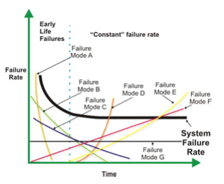Fig. 1. Using Weibull on a complex system requires parsing of individual
failure modes to avoid the “random trap.”

So, let’s look at some data that I generated and analyzed using Weibull analysis. The table in Fig. 2 illustrates four data sets of 10 failure events under four risk profile scenarios – Random (β=1.06), Early Life, (β=0.64), Wearout (β=5.42) and Extreme Wearout (β=16.86).

Refer to the row highlighted in yellow: Under each scenario, the Mean Time Between/To Failure (MTBF/MTTF) is equal to 50.  This was done intentionally to illustrate the effect. Note the extreme difference in the MIN/MAX life for each of the four scenarios.

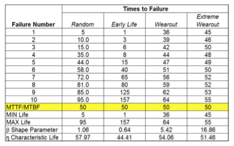Fig. 2. Failure data under four risk-profile scenarios: Each has an MTBF/MTTF of 50,
despite the four of them having very different MIN/MAX ranges.

Now let’s look at the data graphically.

Figure 3 illustrates the cumulative density function graphs for each of the four risk profile scenarios. Figure 4 illustrates the probability-density function graphs for each of the four risk-profile scenarios.

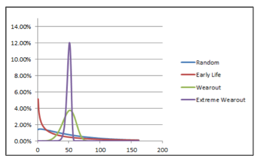Fig. 3. The cumulative number of failure as a function of time/cycle/miles
for each of the four risk-profile scenarios.

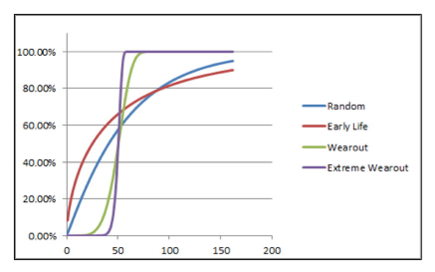Fig. 4. The probability-density function illustrates the distribution of failure risk as a
function of time/cycle/miles for each of the four risk-profile scenarios

.

In all cases, the X-axis is time/cycles/miles or some other usable form of asset utilization. It should be evident, despite the fact the MTBF/MTTF is identical (50) for each of the fours scenarios, that how we approach the various scenarios in this hypothetical plant should be very different.

I have highly simplified Weibull for this article. There’s clearly a great deal more to learn about this tool.  However, a few simple and easy-to-learn Weibull tricks can yield a great deal of value. (The 80:20 rule really does apply here.)

So, let’s  get busy. Start leveraging Weibull analysis to power up reliability at your plant.TRR

ABOUT THE AUTHOR
Drew Troyer has 30 years of experience in the RAM arena. Currently a Principal with T.A. Cook Consultants, he was a Co-founder and former CEO of Noria Corporation. A trusted advisor to a global blue chip client base, this industry veteran has authored or co-authored more than 250 books, chapters, course books, articles, and technical papers, and is popular keynote and technical speaker at conferences around the world. Among other things, he also serves on ASTM E60.13, the subcommittee for Sustainable Manufacturing. Drew is a Certified Reliability Engineer (CRE), Certified Maintenance & Reliability Professional (CMRP), holds B.S. and M.B.A. degrees, and is Master’s degree candidate in Environmental Sustainability at Harvard University. Email dtroyer@theramreview.com.

Tags: failure modes, analysis tools, condition monitoring